Video: Introduction to Dynamic Conditional Correlation (DCC)

Good evening Tino, as suggested I am moving my comment from yt over to this forum and restructured some bits. Thank you in advance for taking the time to share your thoughts on these ideas. I would also love to read your phd thesis on this subject matter if it is available.

Optimizer:
I am using 5min interval intraday data, hence returns are quite small. for instance, a return of 0.001 in absolute terms only converges to 1 when multiplied by a 1000. Doing this works for me in the optimizer, and then dividing conditional vol. by 1000 here:


Is this just or does this raise issues/concerns I am unaware of?

Optimizer Performance&Speed

For context, i am trying to implement this model in an app that models volatility and related risk measures on a real-time basis, hence the interest in faster computation…

Would you say it makes sense to narrow down the a and b parameter bound further in pursuit of a faster optimization time. e.g: bnds = ((0, 0.3), (0, 0.95)).

Other ideas:
-Exchange forloops for vector computations in the ā€˜loglike_norm_dcc_copula’ function
-Resort to multiprocessing although multiprocessing within packages themselves is a bad route to take

Another approach to accelerate the performance would be to trim down the sample. (currently 40000 datapoints for each security for 2yrs of 5min intraday data) Oriented on (Karmakar and Paul 2019, pp.699-709) choice of sample size: Intraday portfolio risk management using VaR and CVaR:A CGARCH-EVT-Copula approach | Request PDF
Option 1:
Trim down the dataset to perhaps only the last month worth of data. My worry here is that volatility could be above or below the mean for some time and that my model parameters would not respect the mean-reverting property of the markets.
Option 2:
Not sure about this one but if i use longer time intervals for returns e.g.30min returns, this forecasts the next 30min vol. so it wouldnt be applicable to accuratly forecast the next 5min return

A last technical question:

On the ā€˜garch_vol_df’, are the last values for garch volatility of the securities in the time series already inherently the forecasted volatility estimate for t+1? Same question for the ā€˜dcc_corr’ df for forecasted correlation respectively…

Thank you in advance for taking the time to answer!

Hello sir, thanks for posting here.
Let me try and answer your questions in order:

The models expect the scale of returns to be: 1.00 representing 1%
Now, at 5 mins you are not gonna get returns in that scale.

The biggest issue you are facing is that GARCH effect are likely not present using 5m intervals. The way trading activity works is U shaped, with all the action at the open and close, with a very thin market during the middle of the trading day.

To jump and answer some of your bits below, this is why Realized Volatility GARCH (RV GARCH) was invented, so it could incorporate intraday data, but not in the way you are currently doing it.

The end goal is to still have a single number being produced each day, which is composed of the aggregation of the intra-day intervals. A simple example would be to sum the squared 5-returns between the open and close.

In this way GARCH effects for the price are still maintained, but you now have an extra piece of information being informed with what path that intraday price took. An extreme and obvious example would be of a stock with opens at $100 and closes at $100. Looking at traditional metrics you would say there has been 0 vol, but you don’t know the path this stock took. It could have been trading at $1 by mid-morning, and then at $1,000,000 just after lunch, and then settling back at $100.

The 5m intervals would capture this vol, even though daily returns are 0.

This is the core topic of my PhD thesis.

Let me attach a few useful papers which helped me, and also my thesis which I did my best to explain everything step by step. As with all these things, there are a ton of auxiliary considerations, such as various distributions, the optimization methods (I use MCMC for example rather than a maximum likelihood optimizer) and what the end goal is; I used GARCH for Value-at-Risk forecasting.

This is a good intro paper to the topic. You can ignore the Skew-t distribution and the VaR bit
Japanese Economic Review 2011 WATANABE.pdf (303.6 KB)

This is my thesis. It gives a slow, step by step build up of the topic. The bit you should look at is page 50 of the PDF, at formulas 3.4 and 3.5, where RV_t-1 is that aggregated intraday component.
My PhD Thesis

Here is a MATLAB file you can take a look at. One day I will convert it to Python :slight_smile:
RV is your aggregated intraday data, r are your daily returns, est contains all your parameters, with

\Theta = [0.05, 0.3, 0.6, -0.1, 0.8, -0.1, 0.1, 0, 0.4, 0.4]

being good starting values. Which bring me to your other question. Absolutely you should impose both restrictions (such as what the possible parameters space that should be searched) and also some parameter bound which either make the model explode or are not allowed, such as negative degrees of freedom etc.
loglike_RV_N_N.m (2.6 KB)

To answer your forecasting question, no, the arch package as I am using it in the DCC notebook is not doing any doing any forecasts, and neither is the DCC.
Pretty straight forward with the package

am = arch_model(rets, dist = 't')
res = am.fit(disp='off')
fcast = res.forecast(horizon=1)
fcast.variance

You will see a column called h.1 which is the 1 step ahead forecast using the data on that day as the latest input. Careful as to gong too far with the forecast, as it’s very noisy. Only 1 step ahead are advisable, as they will just converge to unconditional variance:

var = \omega/(1-\alpha -\beta)

I hope that gives you some food for through.
Cheers,

Tino

Hi Tino,

thank you for your extensive reply! Lots to digest here. I am unable to respond to all the issues you touched on here just yet as it requires more thorough reading on my behalf.

Regarding the intraday periodacity, thank you for pointing this out as i was not aware of the purpose of the rv garch model for instance!
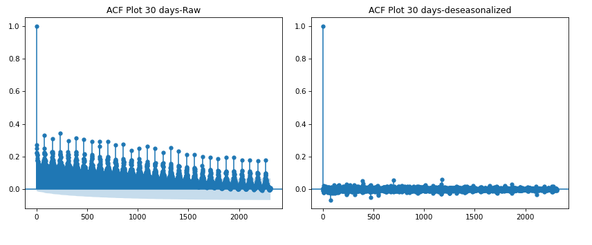
I have taken the intraday periodacity into account beforehand (as i failed to mention beforehand) by differencing absolute returns on each day. The ACF plots show that this has done a good enough job. I am aware that I am probably overlooking a whole bunch of other considerations in the process…

Having processed returns as such, I should be fine to use the deseasonalized data to implement your DCC Garch script as it is…

Thank you a lot for giving me the necessary guidance regarding altering the code to get the forecasted volatility value of the securities. That works for me.

Do you know how the forecasted dcc value can be calculated? The dcceq function takes theta (i have those from the optimization) and trdata. Trdata is calculated from the udata_list. Does this mean i need to forecast a return to get the respective udata_list value to feed this to the dcceq function to get the forecasted dcc value?

I am aware of the long-term convergence to unconditional variance. I am still a bit puzzled on how this could be applied to a daily VaR figure as convergence effects are different depending on the length of trading day remaining. Or if it is even feasible to do so if risk should be assessed on a shorter term basis. Reading both your Phd thesis and the Watanabe paper on forecasting intraday VaR makes me aware that this is not a straight forward thing to do nor is the math easily digestable. I will put more time and thought into it for sure and maybe get back to you with a perhaps more precise question. I assume there is no quick simplistic approach to compute an intraday VaR figure…(i.e. the scope of a 10min youtube video…cheeky pun)

Regarding the function garch_to_u:
Is the purpose of this to transform the t distributed data to a uniform distribution to help the optimizer, or does it serve a different purpose?

udata = t.cdf(std_res, nu)
The udata output confuses me as the udata array does not return values that range from 0 to 1 as i would expect in a cdf.
Some guidance on this would help me a lot!

Best regards from Berlin,

Toni

I think I have understood the last bit better now:

Regarding the function garch_to_u:
the purpose is to transform the standard normalized residuals form the rets to uniform data (t.cdf) in order to later transform them to a normal distribution to apply the normal log likelihood estimation. (norm.ppf)

Is this correct?

Thank you in advance for your help!

1 Like

That is indeed correct. Copulas need uniform distributors as inputs, so we need to transform the residuals coming out of GARCH, the marginal.

We can then pick any distribution we want for the dependency, where I am using Normal for this.

Thank you for getting back to me on this! Regarding the DCC Forecast, i would know how to code the forecasted correlation for a garch (1,1) model. For a Garch(p,q) it becomes challenging due to the n lags in the model. Your code is for pq as the value was not specified i.e. am.fit(p=1, q=1) if i understand correct.

I could dumb the model down to a 1,1 but would love to do it on a pq model

Last question, promised :wink:

Have a great weekend,

Toni

For the forecast, the res item has the values of p and q, or you can override them if you want.
When you setup the model in the first line, the default options are 1,1. This is saved in am, and then once fit, the parameters are saved in res.
In my experience, there is 0 advantage in going beyond 1,1. Just stick to that. Distributions make way more of a difference.

1 Like

Yes I read that a 1,1 is not that bad afterall but great to get your reconfirmation on this! Thank you a lot for all your help!

1 Like

Hi Tino,

Thanks for the great video and the simple explanation of the DCC method.

I am currently in my last semester of my business administration studies and am writing my bachelor’s thesis accordingly. Which examines the correlation of the European stock market (measured by the ā€˜MSCI Europ’) and cryptocurrencies (measured by the ā€˜S&P Cryptocurrency Broad Digital Market Index’) in the 1.5 years before and after the COVID breakout (31.12.2019).

While searching for possible research methods, I stumbled across your video on DCC and am of the opinion that the method is more suitable than static correlation due to the focus on the ā€˜COVID’ event. In my studies, due to my focus on economics, I did not have a deep knowledge of statistics and am only familiar with classical correlation. How difficult do you think it is to learn and thoroughly understand the DCC? Do you think that using DCC as a method adds more value than classical correlation or do you think that by splitting into 2 time series (before and after COVID) classical correlation is sufficient? Another possibility would be to use a rolling correlation.

It would mean a lot and help a lot if you could briefly give me your thoughts on the structure of the study and the appropriate method.

I look forward to more interesting videos in the future.

Best regards from Munich
Sebastian

Hi Sebastian,

Thanks for sharing your experience.

This is a bit of a tough one as there are going to be issues of stationarity.
Anyway, if you want to go down the DCC path, please remember that it’s not magic, but simply a way to incorporate new info on a daily basis, rather than a single number to represent a relationship over years.
It is not too dissimilar to rolling correlation, as it is essentially that but with a decay parameter, so how much of yesterday do we consider, and the day before yesterday etc?

If you believe there should be a structural break in the data, so that 2 models with different parameters would perform better than a single one, then it’s up to you to justify this. COVID certainly made all correlations spike towards 1, as everything was going down at that time.
So what a classic correlation looks like if you divide your data into 2, splitting in on 1 March 2020 for example.

It could also be useful to use 2 DCC models, again splitting the data on 1st March 2020.

I would certainly use DCC if I feel that the extra work is worth it. See what happens and see if the daily correlation number moves around a lot.

Happy to help more. Please let me know your thoughts and findings.

cheers,
Tino

1 Like

Hello Tino!

Thank you for the DCC video overview! I really enjoyed also your other videos, especially since it is difficult to pack advanced content in such a short time-frame. Keep it up! I am investigating volatility modelling in my private time so this is an interesting topic for me. Especially the DCC copula looks interesting as an approach as the DCC/BEKK parameterisations are rigid and costly in parameter space. In the video if I am not mistaken you’re using GARCH(1,1) with t-distributed errors, recovering univariate models’ residuals CDF (from t) and then using a Gaussian copula for the multivariate modelling part. If we wanted to use a skewed-t (I think you also did a video on that one!) for the univariate part, one could fit GARCH(p,q) with skew-t errors and use obtained parameters to get skew-t CDFs for the residuals (perhaps via scipy.stats.nct?). Would there be any other changes required? Also, could you please provide some links to formulas used for the DCC equation section and loglikelihood estimation? I am also curious about a Student-t copula, which would exhibit tail dependence - and the extension from the Gaussian one to Student-t. Do you have some examples or links I can check on how to implement it in the DCC python setup? It seemed to me perhaps one can re-use the DCC normal copula python code (you provided!) and add something extra there for degrees of freedom, so one would have an extra, third parameter (apart from a, b).
Lastly on the forecasting topic, as a suggestion, it would be great if you could do a video explaining univariate and multivariate GARCH forecasting, model evaluation (perhaps in terms of VaR or other statistical tests) and scenario analysis. Thanks! Have a great weekend!

Greeting from Vienna!

N.

1 Like

Hey Nick,

Glad you are liking the videos. So many topics I can cover.

Yes, you are correct, you can change the marginals to use any GARCH model/distribution you like, as long as you convert the residuals back to the correct uniform distribution.

For DCC, you can find all the info in my thesis here.
Look at page 71, you should be able to match the code with the formulas.

The log likelihoods are on page 105 onwards.

I am actually in the process of doing a skewed student-t copula video.

For VaR, again, look at the appendix of the thesis as I cover a lot of that, but again, good video suggestion.

Let me know if you need any more info.

Cheers,

Tino

1 Like

Hi Tino,

Many thanks for your reply and your thesis provided! I will check out the the formulas for DCC and copula log-likelihood functions and try with the Student copula log-likelihood optimization. Will code it in python and have a go!

Just to confirm my understanding, in copula maximum likelihood applications (and standard DCC applications) one performs an estimation of the covariance (or correlation) matrix at each step of the process, between uniform-transformed observations. Also the dependency structure can be estimated via (rank) correlation estimators applied on the data, and then the copula method would be fit to obtain additional skewness or degrees of freedom parameters. In the example you provided, with the DCC setup, both Q (covariance) and R (correlation) are estimated at the initial step, using linear correlation and then updated using DCC updating equation. Are here Q and R matrices being re-estimated at each step (j in range(1, T)) or rather their initial estimates are getting updated via DCC parameters (a, b)? Is my understanding correct? If yes, what are the implications of this approach in your view? Also, could here a rank correlation be applied as well (e.g., Spearman/Kendall) to obtain initial Q and R estimates?
The approach proposed in the video effectively lowers the number of estimated parameters as covariance/correlations parameters are not being estimated during the MLE procedure (vs. for example copula MLE fit procedure). Could you kindly share the rationale behind the approach or provide some reference for this model choice (perhaps in your thesis)?

I am curious in the reducing the number of parameters in such applications and understanding what dimensions can such an approach handle. For example if you are working with 10k risk factor time-series vs. 500k risk factor time-series, the number of estimated parameters (and the ones you need to maintain!) grows pretty fast. Maybe vine or pair copulas could provide needed flexibility for large portfolios of risk factors.

Perhaps a way or idea to tackle time-varying volatility on the univariate modelling level, is to go with a so-called poor man’s GARCH approach: calculate, for each risk factor time-series, the standard deviation in the last, say 20 days, and use this one to scale each return observations in the series by performing a rolling window calculation, always calculation a ratio between the most recent 20 days sample standard deviation and the 20 days standard deviation given the location of the return observation in the time-series (Hull-White describes this approach in detail but they used a GARCH sigma output; Barone-Adesi describes the semi-parametric version with bootstrapping). So that would leave out several parameters shock/persistence) on the univariate GARCH side. Here the rolling window length (parameter) is arbitrary and can be further challenged/tuned. With this however other issues arise as you would need a mechanism to :

  1. convert standardized return observations into uniform / pseudo observations; here I saw a non-parametric rank technique that could come in handy in the following book - Quantitative Risk Management (2015)
  2. perform simulations to analyse scenarios or make forecasts after the copula fitting is performed
  • here I would need to think of something appropriate (perhaps bootstrapping done carefully).

The standardized returns could be analyzed for serial correlation understand whether the transformation was appropriate and if we can have something useful for further analysis steps. Of course, this approach would not capture the stylized facts of financial time-series data a la GARCH - volatility clustering, mean-reversion effects etc.

I know I ask a lot of questions, it’s just modeler’s curiosity, hope you don’t mind!

Aha cool, looking forward to your next video! Have a nice day!

Sincerely,

N.

1 Like

Ah another thing. Browsing through the code I saw you had implemented in your jupyter garch_t_to_u function as below:

def garch_t_to_u(rets, res):
    mu = res.params['mu']
    nu = res.params['nu']
    est_r = rets - mu
    h = res.conditional_volatility
    std_res = est_r / np.sqrt(h) # Do we need np.sqrt() here as it is allready volatility (not variance)?
    # Do you have some reference how should this calculation be performed?
    udata = t.cdf(std_res, nu)
    return udata

Perhaps as a suggestion this part can be simplified using arch package .std_resid method as below:

def garch_t_to_u(rets, res):
    nu = res.params['nu']
    #std_res = res.resid / res.conditional_volatility
    udata = stats.t.cdf(res.std_resid, nu)
    return udata

And for skew t:

def garch_skewt_to_u(rets, res):
    nu = res.params['nu']
    lmda = res.params['lambda']
    udata = stats.nct.cdf(res.std_resid, nu, lmda)
    return udata

Let me know if this helps!

N.

Hi Tino,

I am already well under way in building a Risk Dashboard based on the model.

Code for forecasting the DCC var-covar matrix also works.

I was wondering whether its possible to identify the statistical significance of the a and b parameter:

Statisticial packages like this one in R give that output: time series - Interpretation of DCC GARCH output In R - Cross Validated

Do you have an idea into how that could be on the basis of your code?

Kind regards,

Toni

Edit:

An interesting thing i found out with 5min intraday data is that the model requires roughls more than 60 days to obtain useful parameters. when using around 15 or 30 days, a is 0 and the correlation becomes homoskedastic. papers on intraday and dcc ive read (there are not many) all use 2 year samples. Whats your thought on this? I aim to go rather short in my tradeoff of computational time required and model accuracy

Great to see this thread so lively. Lots of passionate DCC advocates :slight_smile:

1 Like

Hi Tino!

I was playing around with the DCC copula for multivariate t distribution and ended up coding the PDF and log PDF functions from scratch. Only later I found that scipy has it built in and implementing it for the log-likelihood copula function can be done in a straightforward manner, please see below, I’ve re-used the code from your example :blush:

def ll_t_dcc_copula(theta, udata):
    N, T = np.shape(udata)
    llf = np.zeros((T,1))
    _, _, df = theta
    trdata = np.array(stats.t.ppf(udata_list, df).T, ndmin=2)
    Rt, veclRt = dcceq(theta[:2], trdata)

    for i in range(0,T):
        llf[i] = stats.multivariate_t.logpdf(trdata[i,:], None, Rt[:,:,i], df) - stats.t.logpdf(trdata[i,:], df).sum()
    llf = np.sum(llf)
    
    return -llf

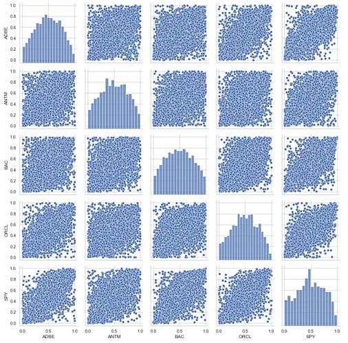
The mean vector was set to None, which simply defaults a zero vector of length N. I’ve performed the estimation on a set of NYSE/NASDAQ stocks and the parameters looked plausible, given the nature and volatility of the underlying log-returns. What I was curious about, when inspecting GARCH-t transformed log-return pairs, prior to fitting the t-Copula. Their histograms looked somewhat off, as if the transformation did not result in the desired uniform property, please see image below:

What does this look like to you? I’ve fitted each time-series with a univariate GARCH (1,1) model, with t distributed errors. The transformation to uniform observations was performed by a modification of the function you provided, please see below:

def garch_t_to_u(rets, res):
    nu = res.params['nu']
    udata = stats.t.cdf(res.std_resid, nu)
    return udata

Here the only change is that I am using the arch package std_resid method, which generates the so-called devolatized time-series, where model residuals are divided by the conditional volatility.

A similar scipy call can be re-used also for the normal Copula log-likelihood, where I’ve made a comparison to your implementation and the log-likelihood sums matched to a decimal point:

def ll_norm_dcc_copula(theta, udata):
    N, T = np.shape(udata)
    llf = np.zeros((T,1))
    trdata = np.array(stats.norm.ppf(udata).T, ndmin=2)
    Rt, veclRt =  dcceq(theta, trdata)

    for i in range(0,T):
        llf[i] = stats.multivariate_normal.logpdf(trdata[i,:], cov=Rt[:,:,i]) - stats.norm.logpdf(trdata[i,:]).sum()
    llf = np.sum(llf)
    
    return -llf

For the skew-t multivariate distribution I presume some work from scratch would be required to code the log-likelihood function for DCC Copula estimation! I will look into the thesis you provided for the appropriate skew-t formulas.
I am now looking into coding an N-day DCC prediction step for the conditional correlations. My idea is to forecast between 30-90 days ahead, but I am fearful errors will start creeping in pretty fast. Do you maybe have a suggestion of a forecast horizon which can provide a reasonable balance ? Many thanks!

Hope this helps! Cheers and have a relaxing weekend!

N.

Hello Toni,

Thank you for the link and question, it is indeed of interest to have an idea about the uncertainty of the parameter estimates. For DCC GARCH testing one can perform tests on both the univariate GARCH and multivariate GARCH fits. For univariate GARCH analysis you can look at the distribution of the standardized residuals and a visual check whether they’re i.i.d. (i.e., the model managed to explain away some stylized facts of financial time-series data). Also a more formal Ljung-Box test for serial correlation can be performed up to some lag. On the other hand, the multivariate distribution choice does not have to fit well, even though the marginals are looking fine. Please see some approaches for multivariate testing in the below text by Orskaug, chapter 8.4:

Also an approach from Alexious Ghalanos (author of rmgarch in R) mentions a multivariate normality test (Mardia), maybe this one could be of interest:

https://bitbucket.org/alexiosg/rmgarch/src/master/R/rmgarch-tests.R

I think inspecting VaR violations would be the proof of pudding. Perhaps here the Kupiec test(binomial) can be of assistance!

Ah regarding the DCC forecasting part I too plan to work on that one at the moment. If you could share you approach/code, for comparison, that would be helpful. Cheers!

Hope this helps. Have a nice weekend!

N.

Hey Nick, Looks like you are making loads of progress on this.
With the DCC, you need a way to establish day 1 correlation, hence why we use just a standard correlation/covariance matrix, and then update it after that.
It’s similar how in GARCH you need a day 1 value to start with, so some sort of sample variance can be used to give you a starting point. It doesn’t matter TOO much, as it will sort itself out after some day iterations anyway, but it’s nice to help the model as much as possible.
For your other questions, looks like they are rhetorical and you have answered them yourself anyway :slight_smile:

With regard to using packages etc, I always prefer writing my own stuff from scratch as you can see exactly what is going on, as sometimes things aren’t what they seem.
For example, if we talk about skewed-t distribution, there are so many implementations. You also learn a whole lot more by converting formulas in papers to code. But that’s just my choice.
another thing is that I like to be very explicit in my code, because when I look at it in 3 months time, I won’t remember what all the cheeky shortcuts did.

With regards to the pair plots, I am not sure why the single stocks aren’t coming out uniform. Very hard to tell from here. Have you tried doing a single one on it’s own, and have a look at the parameters if they are statistically significant etc. GARCH isn’t magic powder, and especially if you include March 2020, some of those returns will be off the charts and break everything. That’s all I can suggest by just looking at that chart.

I am working on skew-t multivariate copula right now, so I can share that code soon.

Hope you had a great weekend too
Ciao

Tino

1 Like

Hey Toni,

so you should be able to get statistical significance of the a and b from the optimiser that you are using, either a ML one or MCMC (my weapon of choice).
With the intraday stuff, are you grouping it up into a single value per day, or are you using that data as is?
With intraday stock returns, you will find all of the action is at the open and close, and very little happening during the middle of the trading day.
I wouldn’t be using straight 5 min returns as if they were daily returns, I don’t think the model was designed for that. Your mileage may vary!

And yes, nice to see a few DCC fans congregate in one place :slight_smile:

Hi Nick,

do apologize for my late reply!

Thanks a lot for taking the time to share your considerations regarding my problem set. I have skimread sum of these approaches and they seem promising. I will explore them in more detail in due course. Its probably beyond the scope of this project to validate the model with backtest implementations. What i thought about was to simply compare the deviation of the forecasted var-covar matrix from t-1 with the realised var-covar matrix as a percentage…But i can surely discuss some of what you suggested in the outlook section of the thesis.

Let me share my code to forecast the var-covar matrix, Ht. The easiest way is to share all which also includes the original code from Tino with some modifications:

*This is written for a 1 step ahead forecast. For more, an additional looping logic would have to be applied using the last forecasted val…

#starting from after loglike_norm_dcc_copula....

#empty list to capture optimized Qtvals
lastQt=[]`
def dcceq(theta,trdata):
   
    T, N = np.shape(trdata)

    a, b = theta


    if min(a,b)<0 or max(a,b)>1 or a+b > .999999:
        a = .9999 - b
        
    Qt = np.zeros((N, N ,T))
    
    
    Qt[:,:,0] = np.cov(trdata.T)
    global Qbar
    Qbar=Qt[:,:,0]  #use qbar outside function for forecast
    Rt =  np.zeros((N, N ,T))
    veclRt =  np.zeros((T, int(N*(N-1)/2)))
    
    Rt[:,:,0] = np.corrcoef(trdata.T)
    
    for j in range(1,T):
        Qt[:,:,j] = Qbar * (1-a-b)
        immediatedisturbances=np.matmul(trdata[[j-1]].T, trdata[[j-1]]) 
        Qt[:,:,j] = Qt[:,:,j] + a * immediatedisturbances
        Qt[:,:,j] = Qt[:,:,j] + b * Qt[:,:,j-1]
        Rt[:,:,j] = np.divide(Qt[:,:,j] , np.matmul(np.sqrt(np.array(np.diag(Qt[:,:,j]), ndmin=2)).T , np.sqrt(np.array(np.diag(Qt[:,:,j]), ndmin=2))))


    for j in range(0,T):
        veclRt[j, :] = vecl(Rt[:,:,j].T)


    #capture last optimized qt value of timeseries
    Qt_end = Qt.flatten()
    Qt_end=Qt_end[(len(rets)-1)::len(rets)] #syntax: start:stop:step
    Qt_end=Qt_end.tolist()
    lastQt[0:(numvars**2)]=Qt_end #optimizer loops through function several times, only Qt vector of final and optimum outcome should be used for the forecast   
    

    return Rt, veclRt


#this function takes returns, applys a garch model to it with a t distribution, then calls the function garch_t_to_u
model_parameters = {}
udata_list = []
fcast_conditionalvariance_list = []

def run_garch_on_return(rets, udata_list, model_parameters):
    for x in rets: #forloop iterates through rets columns
        am = arch_model(rets[x], dist = 't', p=1, q=1) #garch(1,1) model with t-distribution
        res = am.fit(disp='off') #regression output of tickers in rets df
    
        
        #uniformly distributed standardized residuals of return series
        udata = garch_t_to_u(rets[x], res) #garch t_to_u_function call to change garch t volatility to uniform garch volatility
        udata_list.append(udata)
        
        #forecast variance for t+1 / needed for vector Dt in forecastingDCC function
        fcastvariance =  res.forecast(horizon=1, reindex=False).variance
        fcastvariance=fcastvariance['h.1'].iloc[0]
        fcast_conditionalvariance_list.append(fcastvariance/optimizerscaling) #scaled back by 1000 as rets are scaled for the optimizer
        
           
    return udata_list, model_parameters, fcast_conditionalvariance_list

#1.Run Garch on Returns
#2.Estimate dcc theta vals.
#3.Forecast conditional variance of assets
#4.Forecast conditional correlation
#5.Derive forecasted conditional variance-covariance matrix

#1.Run Garch on Returns
udata_list, model_parameters, fcast_conditionalvariance_list = run_garch_on_return(rets.iloc[:,:numvars].dropna(), udata_list, model_parameters)

#2.Estimate dcc theta vals.
#optimizer constraints and bounds
cons = ({'type': 'ineq', 'fun': lambda x:  -x[0]  -x[1] +1})
bnds = ((0, 0.5), (0, 0.9997))
#minimize loglikelihood


#slsqp algorithm as cons and bnds exist. 
%time opt_out = minimize(loglike_norm_dcc_copula, np.array([0.01, 0.95]), args = (udata_list,), bounds=bnds, constraints=cons)

#theta
a,b=opt_out.x

#3.Forecast conditional variance of assets
#variances for variance-covariance matrix-needed for VaR. Needed for Matrix Dt. Careful, Matrix Dt requires vol not variance
fcast_conditionalvariance_list
Dt=np.sqrt(np.diag(np.array(fcast_conditionalvariance_list)))

#4.Forecast conditional correlation, Rt
listoflists=[]
for i in range(0, len(lastQt), numvars):
    listoflists.append(lastQt[i:i+numvars])
lastQt=np.array(listoflists)

fcast_immediatedisturbances=np.zeros((numvars,numvars))

Qtforecast=Qbar * (1-a-b) + a * fcast_immediatedisturbances + b * lastQt
Qtforecast = np.reshape(Qtforecast, (numvars,numvars))

Rtforecast = np.divide(Qtforecast , np.matmul(np.sqrt(np.array(np.diag(Qtforecast), ndmin=2)).T , np.sqrt(np.array(np.diag(Qtforecast), ndmin=2))))

#5.Derive forecasted conditional variance-covariance matrix, Htforecast
Htforecast=np.matmul(np.matmul(Dt, Rtforecast),Dt)

I should have named Dt to Dtforecast aswell for proper measure aswell as using fcast here, and forecast there…I do apologize.

Your exploration of different copulas also looks very interesting. Unfortunatly, I havent had the time to look into that in great enough debth!

Kind regards,

Toni

1 Like